Optimizations for collective communications primitives (CCP)

Authors: José Duro, Adrián Castelló, Maria Engracia Gomez, Julio Sahuquillo, Enrique Quintana (UPV)

1 Introduction

In this blog entry, we present the characterization of the network congestion for the target RED-SEA applications. This congestion is mainly due to collective communication operations, and therefore some of the optimizations for collective communications primitives (CCP) proposed in Task 3.1 of the RED-SEA project for the reduction of congestion are presented.

In the context of the RED-SEA project with extreme computing and data components, parallel applications will generate large congestion due to collective operations. This means that improvements in the performance of these operations will have a very favorable impact on the performance of the applications that use them.

So, in this blog entry we first characterize the impact on the network of CCP and then we propose optimization mechanisms to increase the performance of them.

2 Network Congestion characterization

In Deliverable D3.1 of the RED-SEA project we presented the characterization of the network congestion scenarios derived from the traffic generated by the target applications of the RED-SEA project (LAMMPS and NEST). We performed this characterization with the goal of acquiring a complete knowledge of congestion behavior caused by the target applications, in order to design the congestion-control mechanisms in WP3 of the RED-SEA project. To perform this characterization, we leveraged traces obtained using the VEF tool when running both aforementioned applications.

2.1 Results

We performed two analyses. First, a static analysis where average performance metrics are obtained from the information available in the VEF traces. From this information, we gather, for each trace, metrics such as the most used collective communication primitives or the distribution of messages and traffic among pairs of processes. This analysis provides useful information, but does not offer insights on how this traffic will behave in the network and the actual congestion that it will generate over time.

To provide insights over the execution, we also performed a dynamic analysis where the VEF traces are leveraged to feed the Sauron simulator in order to observe the evolution over time of key network metrics such as accepted network traffic, network latency, switch queue occupancy, and network throughput.

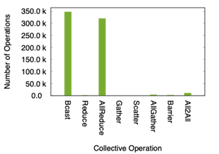
The two applications in RED-SEA exhibit quite a different behavior: LAMMPS relies on a wide variety of primitives, whereas NEST is dominated by the All2All primitive, see Figure 1.

*Figure 1: Number of operations per collective type, 256 tasks (a) LAMMPS (b) NEST*.

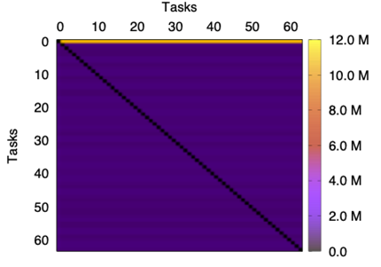
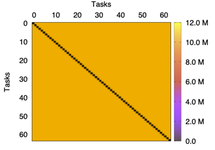
In addition, the message distribution across the network for the two applications is rather different. Specifically, NEST presents a uniform global distribution of messages among source-destination pairs, whereas the traffic distribution in LAMMPS is heterogeneous; see Figure 2 and Figure 3. These figures report the volume of data (bytes) exchanged between pairs of tasks. For LAMMPS, most of the information has task 0 as its source while, in the case of NEST, the distribution is uniform. Note however that this figure illustrates the global behavior for all the traces and, in some moments, the distribution could not be uniform.

*Figure 2 – Bytes transferred between pair of tasks for LAMMPS for the collective operations.*

*Figure 3 – Bytes transferred between pair of tasks for NEST for the collective operations.*

In the dynamic analysis of both applications, we observe that the trace behavior is not uniform over time. On the contrary, it presents a bursty behavior, with time intervals where the network has a low traffic load, and therefore the network latency is low (also the switch queue occupancy), but with other moments where the network experiences a high traffic load. In such cases, the occupancy of the entries of the switch queues increases, the network latency raises, and the network throughput decreases due to congestion. This behavior is due, among others, to the large number of messages generated by the collective communication primitives over a short period of time, and its impact on the network performance.

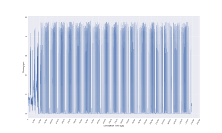
As an example, in the following we compile some plots displaying the dynamic evolution of distinct network metrics over time in order to expose the actual network congestion, as the network traffic generated by the applications is not evenly distributed over time. In other words, in the following plots show how the network behaviour, with a particular configuration, is affected by LAMMPS traces, by tracking the actual congestion in the network over time. For that purpose, the Sauron simulator is fed with the LAMMPS traces to analyse how congestion evolves in the network. We study the traffic transferred in the ports of the network switches, the network latency, the occupancy of the switch buffers, and the network throughput.

Figure 4 presents the evolution of the traffic transferred per time interval at the network ports. For each time interval, the traffic transferred by each port is represented with a different colour, and the traffic transferred at all the ports of a given switch are stacked for the time interval. This means that the peak reached in a time interval is the traffic transferred by the switch in that time interval. We observe that there are time intervals and ports with high transferred traffic, while there are other ports that present time intervals with much lower transferred traffic. This means that the network traffic load has a bursty behaviour, with peaks on demand for some ports and time intervals indicating that congestion can appear at certain points in time. There is an initial phase where the traffic transferred reaches lower values but is more continuous in time than the one transferred in the peaks that are reached later in the traces.

*Figure 4 – Bytes transferred per port (different colour for each port) broken down per time interval (10 us) at switch number zero in an 8-ary 2-tree with deterministic routing for LAMMPS.*

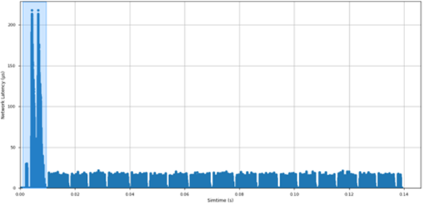
Network latency is a second key network metric that offers insights on congestion and how this problem affects to the network performance. Figure 5 shows the evolution over time of the average network latency per time interval. There is an initial phase in LAMMPS where the network latency reaches values higher than 200 ms. This phase was also present in the previous plot, as a period with low transferred traffic in the network. After that initial phase, LAMMPS presents average latencies per time interval which are below 20 microseconds, with a bursty behavior.

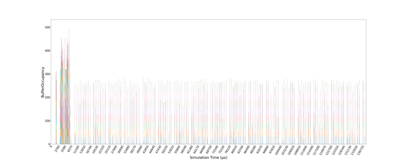
*Figure 5 – Network latency per time interval in an 8-ary 2-tree for LAMMPS with 64 tasks.*

In addition to the metrics corresponding to the traffic transferred and the packet latency, an indicator of the severity of network congestion is the occupancy of the queues at the switches’ ports. Figure 6 shows the queue occupancy evolution per time interval. Each color represents a different network switch. For each switch, we report the highest queue occupancy (i.e., the highest number of busy queue entries) of that switch. The queue occupancies of the different switches are stacked. The maximum queue occupancy for a port is 32. There are time intervals with a high occupancy of the switch queues, especially at the beginning of the trace. This congestion corresponds to the initial part of the trace, where we observed a high network latency and a low transferred traffic. This reveals that there is congestion in the network and that the packets are blocked, not being able to advance through the network. In order to reduce congestion that appears, WP3 will propose solutions based on optimization of collective communications, adaptive routing and injection throttling.

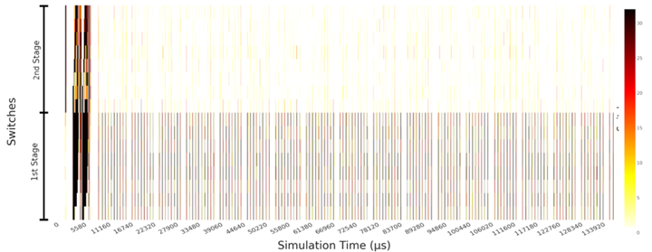
*Figure 6 – Queue occupancy (number of packets in the queue) evolution along time in an 8-ary 2-tree for the whole LAMMPS trace with 64 tasks. Each colour represents a different network switch.*

The same information is represented in Figure 7 in a different way. This plot represents vertically the occupancy of each network switch (the most occupied queue of the switch), according to a colour scale, while the evolution of the occupancy over time is represented horizontally. The topology is a fat-tree with two stages. We observe here that the switch queues in the second stage are much less used than the ones in the first stage.

Figure 7 – Queue occupancy evolution along time in an 8-ary 2-tree for LAMMPS with 64 tasks. Horizontally Vertically all the switches of the network are represented and vertically horizontally how the occupancy evolves along time

Finally, the network throughput evolution is analysed, in order to illustrate the performance attained by the network. Figure 8 shows that, at the beginning of the trace, the network throughput drops to a fifth of its capacity due to the network congestion that is present in the network in that phase (see the previous plots). This occurs in the first phase of LAMMPS, where the switch queue occupancy is high, the network latency is high, and the transferred traffic is low. This means that congestion can severely degrade the network performance.

*Figure 8 – Network throughput evolution along time in an 8-ary 2-tree for LAMMPS with 64 tasks.*

To conclude this congestion characterization, we note that network performance is highly determined by the collective primitives (type and frequency) that each workload involves. More precisely, network performance is determined by the communication patterns defined by the collective primitives of the running workloads. For this reason, as a first step, we analyzed the type, frequency, and communications patterns of the collective communication primitives of the running applications.

3 Software Collective Communication Primitives Optimization

In this section we describe the optimizations of CCPs and after presenting these optimizations we evaluate them.

In Task 3.2, UPV worked toward the software optimization of collective communication primitives (or CCPs) in MPI, improving the performance of the data exchanges over the network. In detail, we analyzed the following techniques in combination with three well-known realizations of the MPI standard, namely OpenMPI, MPICH and IntelMPI:

A performance evaluation of the blocking global reduction (blocking) MPI_Allreduce versus its non-blocking counterpart MPI_Iallreduce immediately followed by the corresponding blocking synchronization MPI_Wait.
An analysis of two realizations of MPI_Iallreduce that offer significantly higher performance when applied to perform a blocking global reduction. These implementations operate by dividing the message (transparently to the user) into either a collection of messages of a specific smaller size or a fixed number of smaller messages, in both cases pipelining the transfers.
A demonstration that splitting the messages to pipeline the transfers benefits not only the global reduction primitive but also other collective operations, such as broadcast or reduce-scatter.
A study of the benefits of an optimal MPI processes to cores mapping. The mapping policies may offer a significant performance loss for some algorithms because they are not aware of where the processes are mapped.

3.1 Mapping policies

Concerning the last optimization, we have considered 4 different mapping policies. The different mappings differ on 2 levels of assignment of tasks to cores (cores and sockets). The first decision is how nodes are selected, if all the cores of a node are used and then a new node is used or first the nodes are selected in a round robin manner assigning just a core in each. And the second level corresponds to the selection of the socket inside the node, first filling the socket or selecting the socket in a round robin manner.

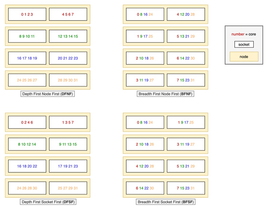
*Figure 9 – The 4 mapping policies evaluated in this task. There are 2 levels of assignments of tasks to cores*.

We have defined 4 different mappings DFNF, DFSF, BFNF, and BFSF (Figure 9). For the Deep variants (the ones that start with D), we populate the nodes first while in the breath counterpart (B) we assign the processes to nodes in a round robin dispatch. In the case of Node First, we fill the sockets while in the case of socket first, we assign the processes alternatively in each socket.

3.2 Performance Evaluation

This section evaluates some of the mechanisms proposed in task T3.2. We start with the evaluation of the several MPI algorithms available in the MPI library to show the high impact that they have. Then we assess the performance of MPI primitive pipelining and finally we evaluate the impact of the task mapping policy on the CCP performance.

3.2.1 Evaluation of MPI algorithms

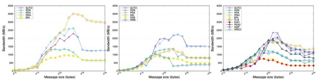
For our evaluation, we employed OpenMPI 4.1.0rc, MPICH 3.3.1, and IntelMPI 2020. The cluster platform for these experiments consisted of 9 nodes equipped with 2 Intel Xeon Gold 5120 CPUs (14 cores each, for a total of 28 cores per node) running at 2.20 GHz, 192 GB of DDR4 RAM. The nodes were connected via an InfiniBand EDR network with a link latency of 0.5 microseconds and a link bandwidth of 100 Gbps. In Figure 10, the X-axis corresponds to message size (in bytes) and the Y-axis shows the bandwidth (calculated as the division of the message size in Mbytes by the time in seconds). This metric offers a bounded version of the execution time providing a fair option to compare the distinct algorithms.

Figure 10 – Performance of the algorithms in OpenMPI, MPICH, and Intel MPI for MPI_Iallreduce using 8 odes connected via EDR network.

3.2.2 Pipelining of message exchanges

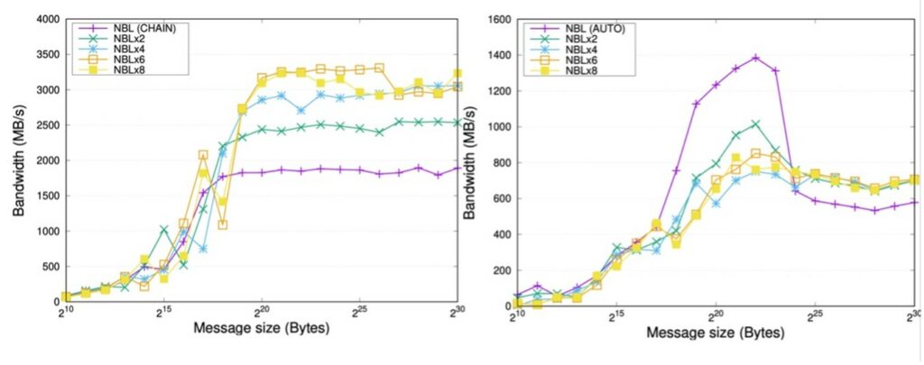
In order to obtain a pipelined variant of the global reduction, we divided (that is, partition or segment) the original message, consisting of s bytes, into several segments (or chunks) of segsize bytes each (except, possibly, for the last one), and performed numseg=ceil(s/segsize) consecutive invocations to the non-blocking MPI_Iallreduce CCP (that is, one per segment), to initiate the exchange of the corresponding segment. An alternative to obtain a pipelined realization of MPI_Iallreduce is to divide the message into a fixed number of smaller messages. For that purpose, we performed the global reduction of a message, of s bytes, by means of numseg calls to the non-blocking MPI_Iallreduce CCP, one per segment of segsize=s/numseg bytes (except for the last one, which has to take into account the possibility of the message size not being an integer multiple of the number of segments). Therefore, the number of primitives which are concurrently executed in this scheme is fixed. Note that the blocking behaviour can be achieved by simply invoking the synchronizing MPI_Waitall function.

Figure 11 (left) reports the effect of pipelining with a fixed message size, applied to the Ring algorithms in OpenMPI for 8 nodes. In the plots there, the purple line corresponds to the non-segmented approach while the rest of lines represents the segment size or the number of segments depending on the type of pipelining technique. For this algorithm, dividing the message into several segments preserves the asymptotic communication throughput at 4,000~MB/s, whereas the original primitive falls from a peak of 3,500~MB/s to 3,000~MB/s or less for large messages.

Figure 11 (right) illustrates the impact of pipelining with a fixed degree of concurrency. The pipelined ring algorithm already improves the performance for messages of size larger than 2MB. In addition, these charts expose that it is possible to accelerate the throughput by up to 25% applying this type of pipelining.

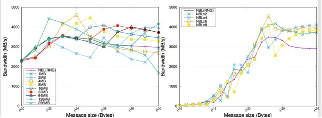
Figure 11 – Performance of the Ring algorithm in OpenMPI with two pipelining approaches. The label NBL(RNG) is the original MPI_Iallreduce ring algorithm implementation using 8 nodes connected via EDR network.

Figure 12 shows the effect on performance of message segmentation for two other asynchronous CCPs from OpenMPI: MPI_Ibcast (left plot), MPI_Ireduce_scatter, and (right plot), showing the generality of the pipelining technique.

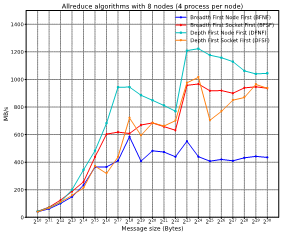
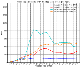
Figure 12 – Performance of the MPI_Ibcast and MPI_Ireduce_scatter CCPs OpenMPI with the fixed number of segment pipelining approach using 8 nodes connected via EDR network. The label NBL(XXX) corresponds to the original realization.

3.2.3 Mapping policies

Figure 13 and Figure 14 show how each mapping offer different performance for different message sizes. Please, notice that the results are employing the best algorithm for each message size. As can be seen in the figures, the best mapping policy is the one that first fills cores of a node and inside the node first fulfil cores of a socket and then the next socket. That is, the closer the neighboring tasks are, the better the obtained results will be.